Imscript is a collection of simple programs for doing image processing in a Unix environment.
This is just vanilla unix philosophy with some specificities for images:
Notice that imscript programs will read any common image format, but will only write asc, pnm, png, and tiff.
1. Filters: read one image and write one image of the same size
	- blur: convolve an image by a shift-invariant user-specified kernel
	- morsi: apply a morphological operation with a user-specified element
	- qeasy: re-scale the dynamic range of an image
	- qauto: re-scale the dynamic range of an image, automatically
	- palette: colorize a grayscale image using a palette
	- dither: binarize an image by error diffusion
	- iion: copy named input to named output (useful to change file format)

2. Accumulators: combine several images into one
	- plambda: apply an arbitrary pixel-wise expression, given explicitly
	- veco: generic pixel-wise expressions for gray images, gray output
	- vecov: generic pixel-wise expressions for color images, color output
	- vecoh: generic pixel-wise operations for gray images, color output
	- tbcat: concatenate images top-bottom
	- lrcat: concatenate images left-right

3. Queries: extract data from one image
	- imprintf: print a formatted string of image data
	- ghisto: common histogram
	- contihist: continuous histogram
	- viewflow:  represent a vector field using a color code
	- flowarrows: represent a vector field using arrows

4. Interpolators: fill-in the holes of one image
	- nnint: nearest neighbor interpolation
	- bdint: interpolation from the boundary of each hole
	- simpois: poisson, laplace and biharmonic interpolators
	- amle: absolutely minimizing lipschitz extension

5. Rescalers: produce an image of different size or shape
	- downsa: zoom out by combining blocks of pixels
	- upsa: zoom in by interpolation inside cells
	- ntiply: zoom in by pixel replication
	- imflip: rotate or transpose the image domain
	- homwarp: apply an arbitrary homography to the image domain

6. Frequecy domains:
	- fft: discrete Fourier transform (direct)
	- ifft: discrete Fourier transform (inverse)
	- dct: discrete cosine transform
	- dht: discrete Hartley transform

7. Point processing:
	- pview: display points or matches as an image
	- ransac: generic ransac implementation
	- srmatch: multi-scale sift matching for registration
	- plyflatten: project 3D points into a 2.5D representation
	- colormesh: build 3D mesh from calibrated 2.5D representation
	- ijmesh: build 3D mesh from non-calibrated 2.5D representation

8. Multi-program suites:
	- siftu: operations for sift keypoints
	- tiffu: operations for tiff files
	- fontu: operations for bitmapped fonts

9. Miscellaneous:
	- synflow: generate a synthetic optical flow field
	- ccproc: connected component filtering
	- ihough2: generic hough transform (for straight lines)
	- tdip: cylindrical hough transform (for sinusoids)
	- rpc_pm: patch match in the altitude domain
	- distance: distance function to a given set of points
	- sdistance: signed distance to the boundaries of a binary image
	- ppsmooth: periodic + smooth image decomposition
	- pmba2: poor man bundle adjustment
	- tcregistration: register two images by translation

10. Interactive programs:
	- fpan: display an image with panning, zooming, and contrast changes
	- fpantiff: like fpan, but understands image pyramids
	- rpcflip: display several calibrated satellite images
	- powerkill: fourier-domain band-pas filter editor
	- epiview: visualize the epipolar geometry between two images
	- viho: interactive homographic visualization
	- dosdo: look at an image and its fourier transform
	- icrop: interactive crop
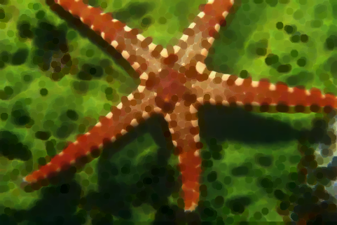
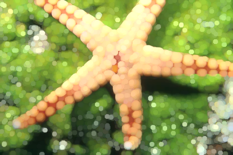
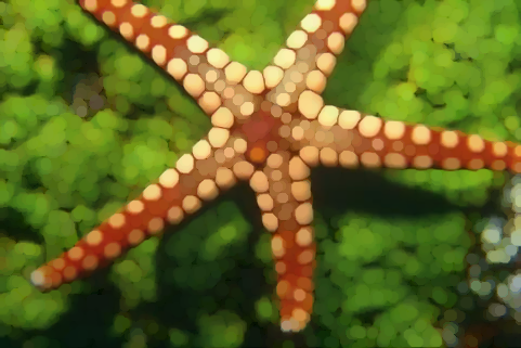
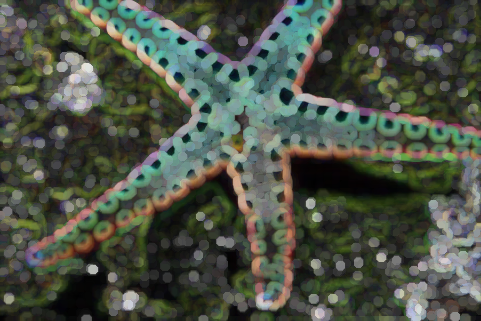
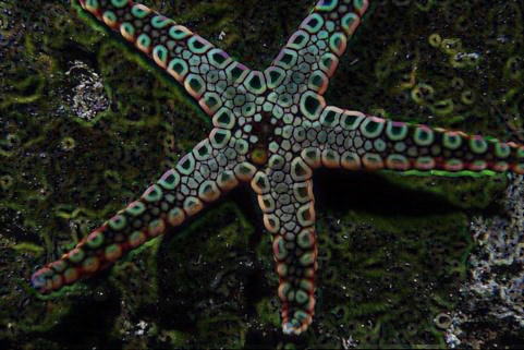
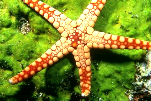
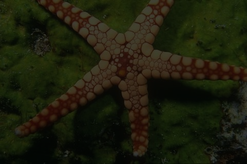
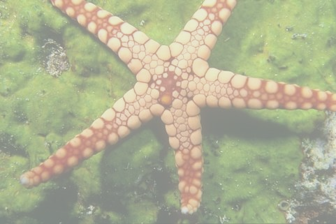
Gaussian blur of different sizes
blur gaussian 1 A.png A_gaussian_1.png
blur gaussian 3 A.png A_gaussian_3.png
blur gaussian 8 A.png A_gaussian_8.png
Gaussian blur with different boundary conditions:
blur gaussian 5 -s A.png A_gaussian_5_s.png    # symmetric boundary
blur gaussian 5 -p A.png A_gaussian_5_p.png    # periodic boundary
blur gaussian 5 -z A.png A_gaussian_5_z.png    # zero boundary
Blur with different kernels of the "same" width:
blur square  11 A.png A_s.png
blur gaussian 5 A.png A_g.png
blur laplace  5 A.png A_l.png
blur disk     5 A.png A_d.png
blur cauchy   2 A.png A_c.png
blur inverse  1 -p A.png | qauto -i -p 1 - A_i.png
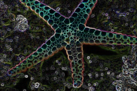
morsi cross: morphological operations with a cross structuring element:
morsi cross erosion       A.png A_x_erosion.png
morsi cross dilation      A.png A_x_dilation.png
morsi cross median        A.png A_x_median.png
morsi cross opening       A.png A_x_opening.png
morsi cross closing       A.png A_x_closing.png
morsi cross gradient      A.png A_x_gradient.png
morsi cross igradient     A.png A_x_igradient.png
morsi cross egradient     A.png A_x_egradient.png
morsi cross laplacian     A.png | qeasy 40 -40 - A_x_laplacian.png
morsi cross enhance       A.png A_x_enhance.png
morsi cross tophat        A.png | qeasy  0 60 - A_x_tophat.png
morsi cross bothat        A.png | qeasy  0 60 - A_x_bothat.png
morsi cross oscillation   A.png | qeasy  0 60 - A_x_oscillation.png
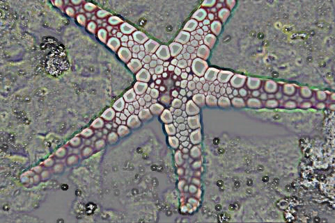
morsi disk5: morphological operations with disk structuring element of radius 5 pixels:
morsi disk5 erosion       A.png A_d5_erosion.png
morsi disk5 dilation      A.png A_d5_dilation.png
morsi disk5 median        A.png A_d5_median.png
morsi disk5 opening       A.png A_d5_opening.png
morsi disk5 closing       A.png A_d5_closing.png
morsi disk5 gradient      A.png A_d5_gradient.png
morsi disk5 igradient     A.png A_d5_igradient.png
morsi disk5 egradient     A.png A_d5_egradient.png
morsi disk5 laplacian     A.png | qeasy 90 -90 - A_d5_laplacian.png
morsi disk5 enhance       A.png A_d5_enhance.png
morsi disk5 tophat        A.png | qeasy 0 100 - A_d5_tophat.png
morsi disk5 bothat        A.png | qeasy 0 100 - A_d5_bothat.png
morsi disk5 oscillation   A.png | qeasy 0 100 - A_d5_oscillation.png
qeasy: linear contrast change with manually chosen parameters:
qeasy 20 200   A.png A_saturated.png
qeasy 0 1000   A.png A_darkened.png
qeasy -300 300 A.png A_bleached.png
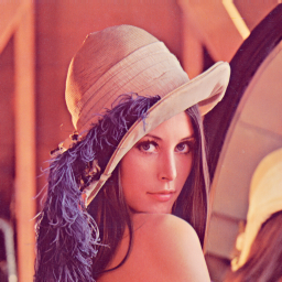
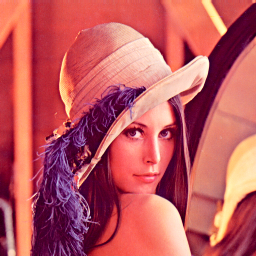
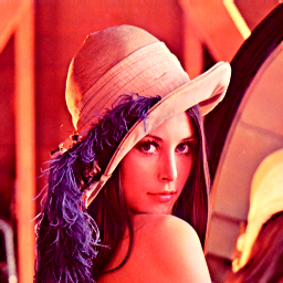
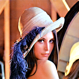
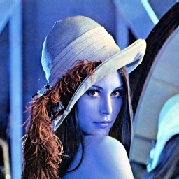
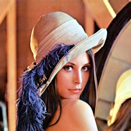
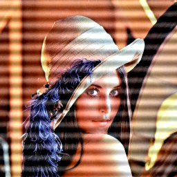
qauto: linear contrast change with automatically chosen parameters:
qauto       lenac.png lenac_qauto.png
qauto -p 10 lenac.png lenac_qauto_p10.png
qauto -i    lenac.png lenac_qauto_i.png
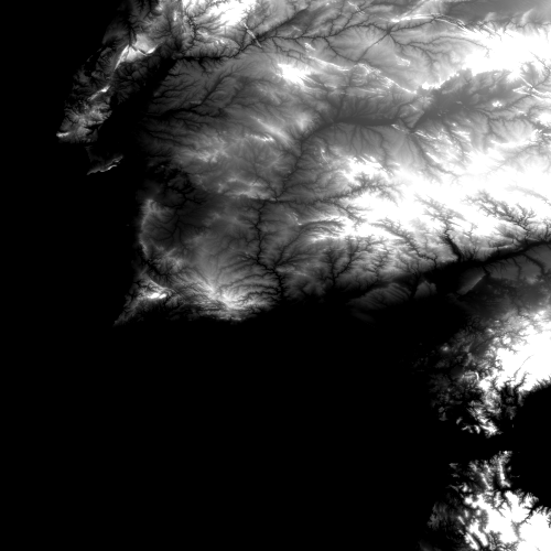
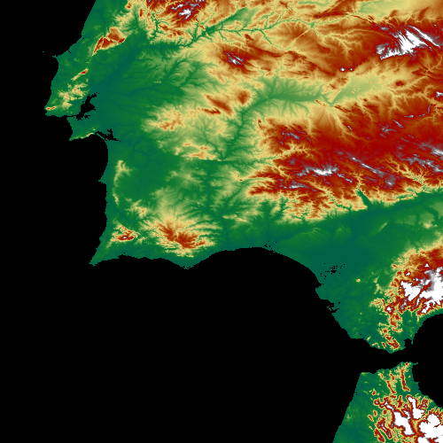
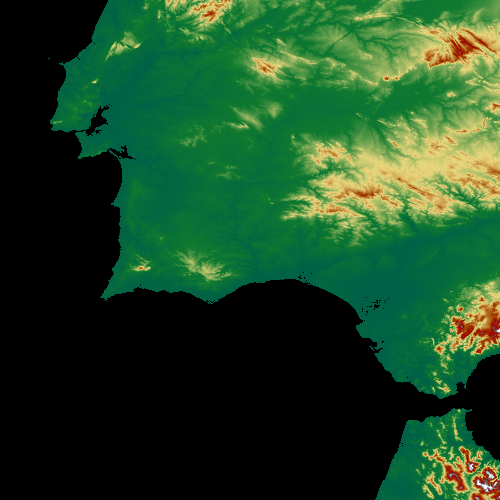
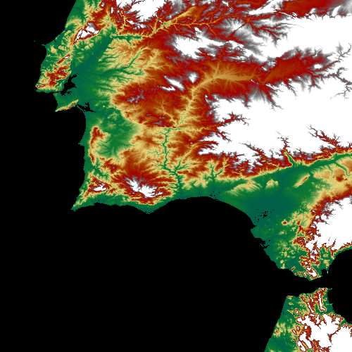
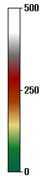
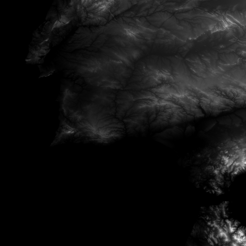
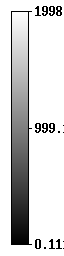
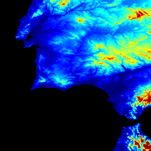
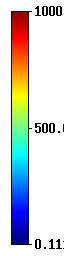
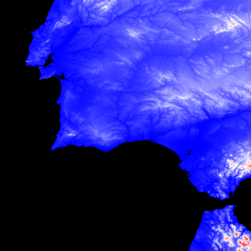
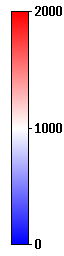
palette: apply a palette to a scalar-valued image (the -l option is optional and writes the associated legend). The palette name can be a pre-defined palette or a gimp palette file:
qauto X.tif X.png
palette 0 1000 dem       X.tif X_dem1000.png    -l leg_dem1000.png
palette 0 2000 dem       X.tif X_dem2000.png    -l leg_dem2000.png
palette 0  500 dem       X.tif X_dem500.png     -l leg_dem500.png
palette nan nan gray     X.tif X_gray.png       -l leg_gray.png
palette nan 1000 jet.gpl X.tif X_jet.png        -l leg_jet.png
palette 0 2000 nice      X.tif X_nice.png       -l leg_nice.png
palette 0 2000 nnice     X.tif X_nnice.png      -l leg_nnice.png
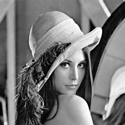
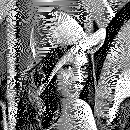
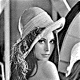
dither: halftoning by error diffusion:
dither lena.png lena_dithered.png
blur C 1 lena.png | qauto | dither - lena_dithered_c.png
plambda: apply an arithmetic expression with input images (the
expression is written in reverse polish
notation). Common arithmetic operators and all functions from
math.h are allowed.
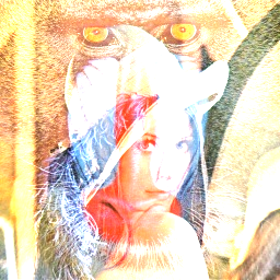
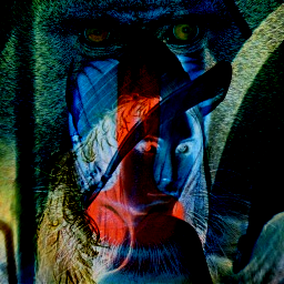
plambda a.jpg b.jpg +        -o ab_sum.png
plambda a.jpg b.jpg -        -o ab_dif.png
plambda a.jpg b.jpg "*"      -o ab_mul.png
plambda a.jpg b.jpg /        -o ab_div.png
plambda a.jpg b.jpg "+ 2 /"  -o ab_avg.png
plambda a.jpg b.jpg "* sqrt" -o ab_geo.png
plambda a.jpg b.jpg fmin     -o ab_min.png
plambda a.jpg b.jpg fmax     -o ab_max.png
The plambda language allows many operations, even when applied to a single image. See the external plambda tutorial for a comprehensive description. Here are some silly examples:
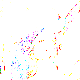
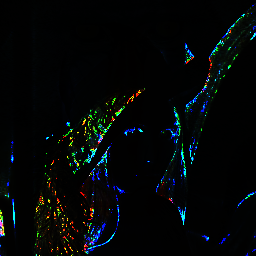
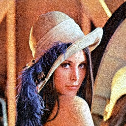
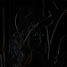
plambda b.jpg "a[2] a[1] a[0] join3" -o b_bgr.png     # swap colors
plambda b.jpg "a[0] a[1] a[2] join3" -o b_rgb.png     # do nothing
plambda b.jpg "randg 20 * +"         -o b_noisy.png   # add luminance noise
plambda b.jpg "a(1,0) a -"           -o b_dx.png      # x-derivative
plambda b.jpg "a(1,0) a - 127 +"     -o b_dx_127.png  # x-derivative plus 127
plambda b.jpg a,x                    -o b_dx_alt.png  # x-derivative (easier)
plambda b.jpg "a,x a,y hypot 2 *"    -o b_edges.png   # gradient norm
plambda b.jpg ":y 50 * sin 50 * +"   -o b_bands.png   # sine of y plus image
plambda b.jpg ":r 50 * sin 50 * +"   -o b_rings.png   # sine of r plus image
plambda b.jpg ":i 8 fmod not  :j 30 fmod not  or 99 * +" -o b_grid.png
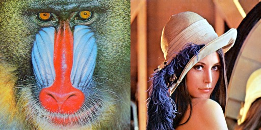
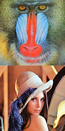
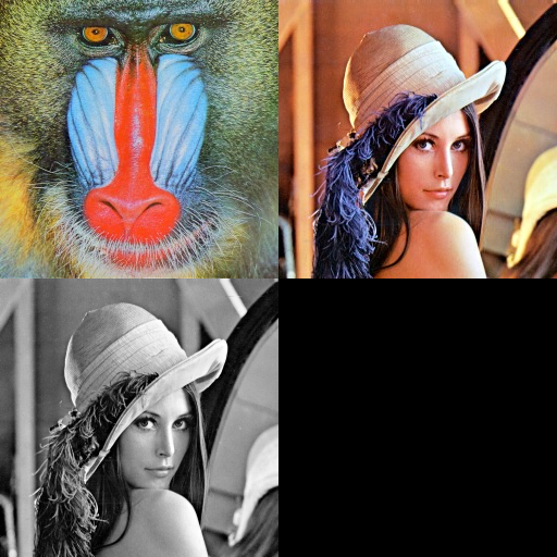
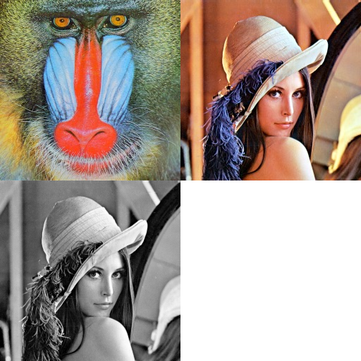
The lrcat and tbcat programs concatenate images horizontally or vertically. The images need not be of the same size. Any missing space is filled-in by the value on the environment variable BACKGROUND.
lrcat a.jpg b.jpg -o ab_lr.png
tbcat a.jpg b.jpg -o ab_tb.png
lrcat a.jpg b.jpg | tbcat - lena.png -o ab_montage.png
lrcat a.jpg b.jpg | BACKGROUND=255 tbcat - lena.png -o ab_montage2.png
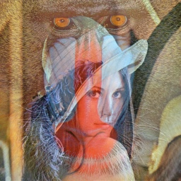
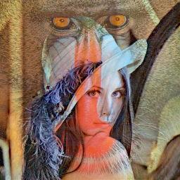
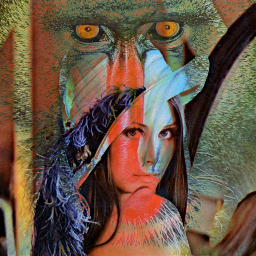
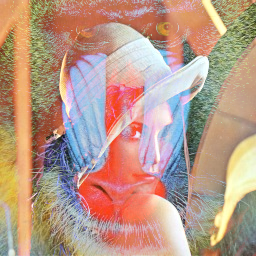
The vecov program aggregates the pixel values of many images.
vecov avg pRi*.jpg -o outv_avg.png
vecov min pRi*.jpg -o outv_min.png
vecov max pRi*.jpg -o outv_max.png
vecov med pRi*.jpg -o outv_med.png      # geometric medoid
vecov modc pRi*.jpg -o outv_modc.png    # component-wise mode
The veco program is similar, but it only works for gray-scale images and supports a much larger variety of accumulators (including very fancy ones).
veco max gpRi*.jpg -o out_max.png
veco euc gpRi*.jpg -o out_euc.png                # euclidean mean
veco avg gpRi*.jpg -o out_avg.png                # arithmetic mean
veco geo gpRi*.jpg -o out_geo.png                # geometric mean
veco har gpRi*.jpg -o out_har.png                # harmonic mean
veco min gpRi*.jpg -o out_min.png
veco lav gpRi*.jpg -o out_lav.png                # logarithmic average
veco lse gpRi*.jpg -o out_lse.png                # log-sum-exp (soft max)
veco mod gpRi*.jpg -o out_mod.png                # mode
veco med gpRi*.jpg -o out_med.png                # median
veco q25 gpRi*.jpg -o out_q25.png                # first quartile
veco q75 gpRi*.jpg -o out_q75.png                # third quartile
veco rnd gpRi*.jpg -o out_rnd.png                # random sample
veco std gpRi*.jpg | qeasy 0 20 - out_std.png    # standard deviation
veco iqd gpRi*.jpg | qeasy 0 20 - out_iqd.png    # interquartile distance
The vecoh program also works with gray-scale images and it finds clusters of values at each pixel. The output is a 8-dimesional image, on the first component the number of clusters, and on the rest, the cluster centers.
vecoh kmeans    gpRi*jpg | plambda - "x[0] 0 4 qe" -o kmeans_count.png
vecoh kmedians  gpRi*jpg | plambda - "x[0] 0 4 qe" -o kmedians_count.png
vecoh contrario gpRi*jpg | plambda - "x[0] 0 4 qe" -o contrario_count.png
vecoh kmeans    gpRi*jpg | plambda - "x[1]"        -o kmeans_k1.png
vecoh kmeans    gpRi*jpg | plambda - "x[2]"        -o kmeans_k2.png
vecoh kmeans    gpRi*jpg | plambda - "x[3]"        -o kmeans_k3.png
vecoh kmeans    gpRi*jpg | plambda - "x[4]"        -o kmeans_k4.png
vecoh kmedians  gpRi*jpg | plambda - "x[1]"        -o kmedians_k1.png
vecoh kmedians  gpRi*jpg | plambda - "x[2]"        -o kmedians_k2.png
vecoh kmedians  gpRi*jpg | plambda - "x[3]"        -o kmedians_k3.png
vecoh kmedians  gpRi*jpg | plambda - "x[4]"        -o kmedians_k4.png
vecoh contrario gpRi*jpg | plambda - "x[1]"        -o contrario_k1.png
vecoh contrario gpRi*jpg | plambda - "x[2]"        -o contrario_k2.png
The imprintf program creates a string from image data. The syntax is very similar to C's printf, with a image-specific set of conversions.
imprintf "Image size=%wx%h avg=%v med=%e min=%i max=%a\n" lena.png
Image size=256x256 avg=119.08 med=119.08 min=0 max=255
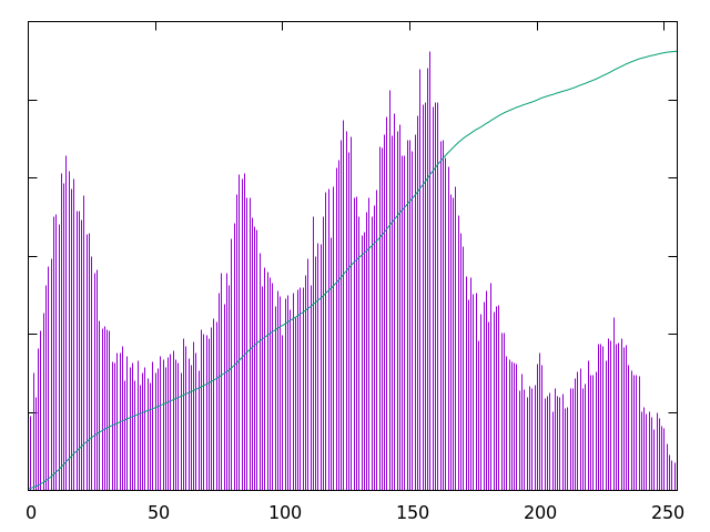
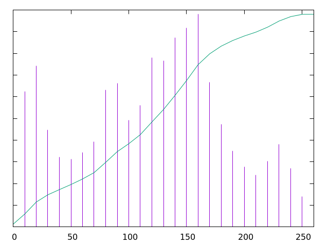
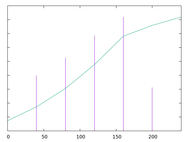
The ghisto program computes the histogram of an image and prints it in a
textual form that gnuplot understands. The -p option produces a
gnuplot file that renders into a png.
plambda lena.png "40 / round 40 *" | ghisto
set xrange [0:240]
set yrange [0:]
set format y ""
unset key
plot "-" w impulses title "histogram", "-" w lines title "accumulated histogram"
	0	5903
	40	7993
	80	10559
	120	13691
	160	16375
	200	6243
	240	4772
end
	0	1474.94
	40	3472.09
	80	6110.39
	120	9531.26
	160	13622.8
	200	15182.7
	240	16375
end
cat lena.png                        | ghisto -p | gnuplot > lena_ghisto.png
plambda lena.png "10 / round  10 *" | ghisto -p | gnuplot > q10lena_ghisto.png
plambda lena.png "40 / round  40 *" | ghisto -p | gnuplot > q40lena_ghisto.png
blur g 0.4 lena.png                 | ghisto -p | gnuplot > glena_ghisto.png
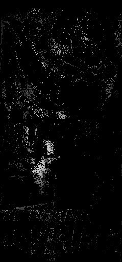
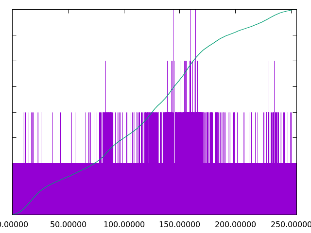
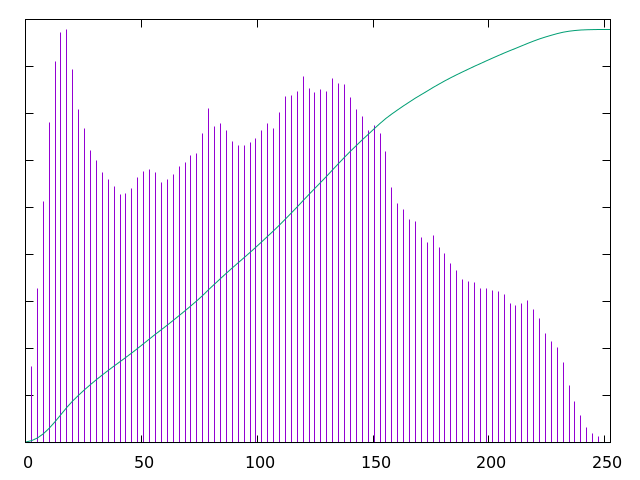
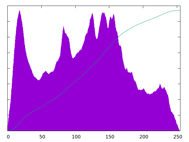
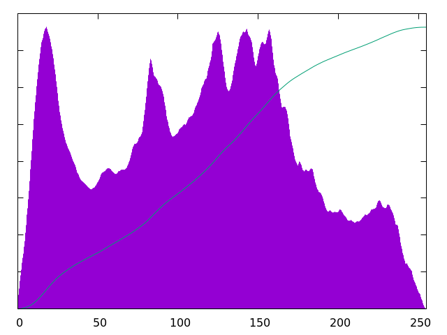
The contihist program computes the continuous histogram of an image (defined as the derivative of the area of level sets of the interpolated image). This is a real-valued function of a real variable, and you have to specify the number of samples to represent this function function and the desired range.
cat lena.png | contihist   100  0 255  - -p | gnuplot > lena_contih_100.png
cat lena.png | contihist  1000  0 255  - -p | gnuplot > lena_contih_1000.png
cat lena.png | contihist  2000  0 255  - -p | gnuplot > lena_contih_2000.png
cat lena.png | contihist 10000  0 255  - -p | gnuplot > lena_contih_10000.png
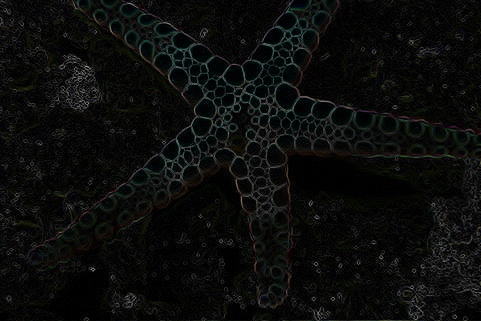
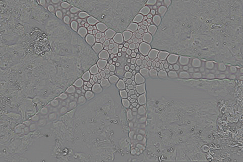
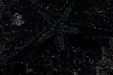
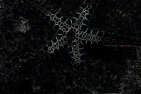
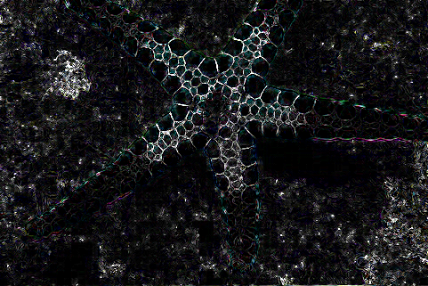
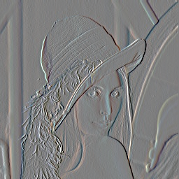
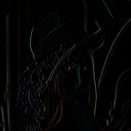
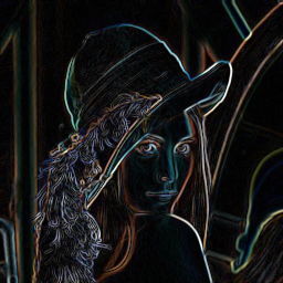
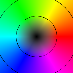
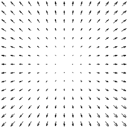
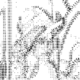
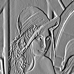
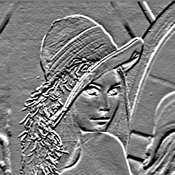
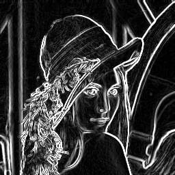
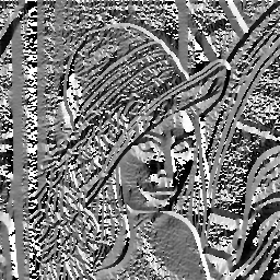
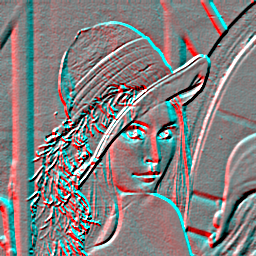
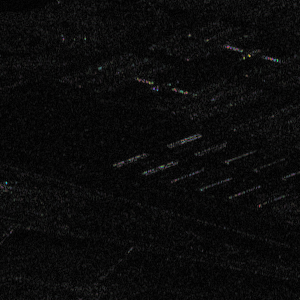
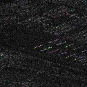
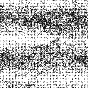
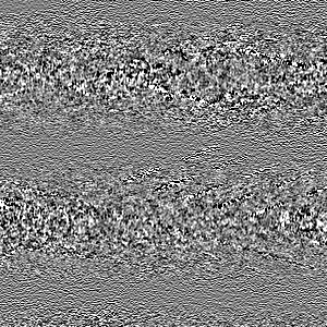
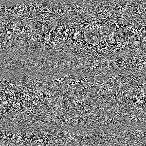
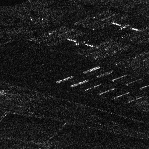
Images with two-dimensional pixels are very important in image processing. They can be for example displacement fields, velocity fields, gradients of gray-valued images, complex-valued images (such as SLC radar images, or Fourier transforms of gray-valued images). Depending on the context, several different visualizations are preferred.
cat wheel.tiff | viewflow  0                                  - wheel_colors.png
cat wheel.tiff | viewflow -1                                  - wheel_lines.png
cat wheel.tiff | flowarrows 0.2 17                            - wheel_arrows.png
cat wheel.tiff | plambda x[0]              | qeasy -1    1    - wheel_x.png
cat wheel.tiff | plambda x[1]              | qeasy -1    1    - wheel_y.png
cat wheel.tiff | plambda vnorm             | qeasy  0    2    - wheel_abs.png
cat wheel.tiff | plambda "x[1] x[0] atan2" | qeasy -3.14 3.14 - wheel_arg.png
cat wheel.tiff | plambda "split dup join3" | qeasy -2    2    - wheel_xyy.png
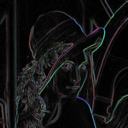
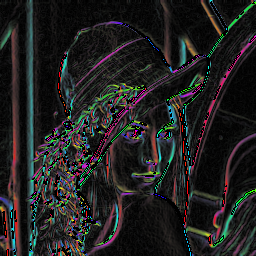
plambda lena.png x,g | viewflow  0                                - g_colors.png
plambda lena.png x,g | viewflow -50                               - g_lines.png
plambda lena.png x,g | flowarrows 3 5                             - g_arrows.png
plambda lena.png x,g | plambda x[0]                       | qauto - g_x.png
plambda lena.png x,g | plambda x[1]                       | qauto - g_y.png
plambda lena.png x,g | plambda vnorm                      | qauto - g_abs.png
plambda lena.png x,g | plambda "x[1] x[0] atan2"          | qauto - g_arg.png
plambda lena.png x,g | plambda "split dup join3"          | qauto - g_xyy.png
cat slc.tiff | viewflow  0                                - slc_colors.png
cat slc.tiff | viewflow -500                              - slc_lines.png
cat slc.tiff | flowarrows 3 5                             - slc_arrows.png
cat slc.tiff | plambda x[0]                       | qauto - slc_x.png
cat slc.tiff | plambda x[1]                       | qauto - slc_y.png
cat slc.tiff | plambda vnorm                      | qauto - slc_abs.png -p 0.1
cat slc.tiff | plambda "x[1] x[0] atan2"          | qauto - slc_arg.png
cat slc.tiff | plambda "split dup join3"          | qauto - slc_xyy.png
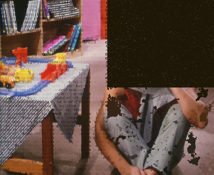
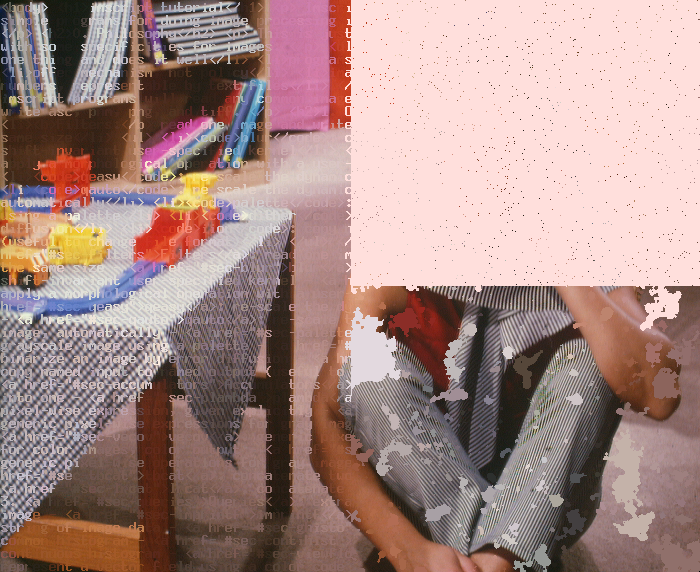
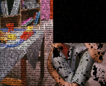
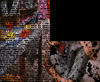
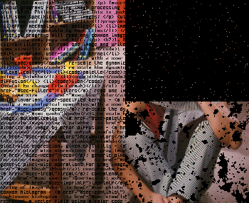
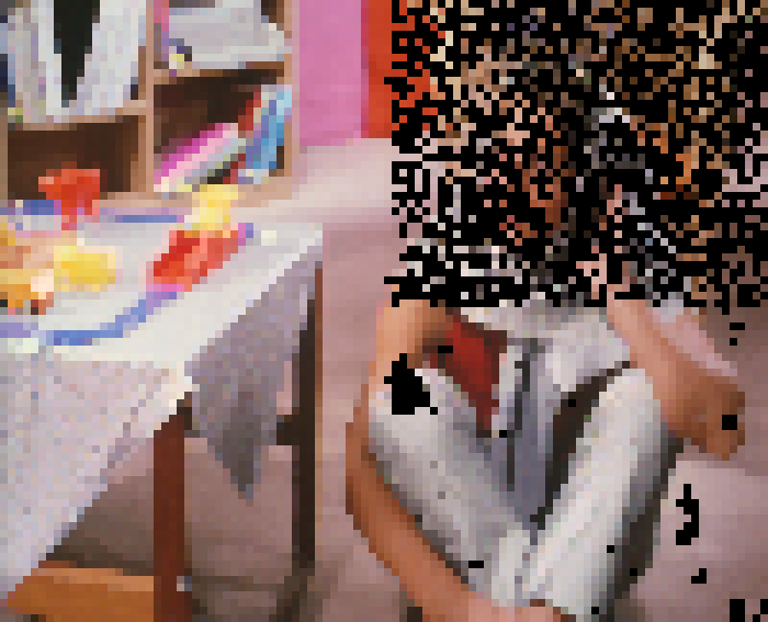
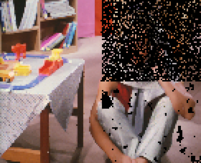
These interpolating filters are used to fill-in the missing values of an image (by default, indicated by a floating point NAN).
qeasy 0 255 masked.tif masked.png
cat masked.tif | nnint             - out_nnint.png        # nearest-neighbor
cat masked.tif | bdint -a min      - out_bdmin.png        # boundary minimum
cat masked.tif | bdint -a max      - out_bdmax.png        # boundary maximum
cat masked.tif | bdint -a avg      - out_bdavg.png        # boundary average
cat masked.tif | simpois          -o out_laplace.png      # harmonic
cat masked.tif | simpois -t -0.08 -o out_biharm.png       # biharmonic
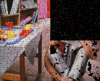
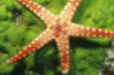
Zoom-in is a particular case of interpolation when the data values are on a regular grid. Zoom-out is a very different problem, typically achieved by filtering the input image and then sampling it at a coarser grid.
The downsa program creates a smaller image by combining blocks of n×n pixels into one. The first argument is the rule to combine several pixel values into one. The rule is specified by a single letter:
downsa v 2 masked.png downsa_avg_2.png  # zoom-out by 2x2 blocks aVerage
downsa i 2 masked.png downsa_min_2.png  # zoom-out by 2x2 blocks mInimum
downsa a 2 masked.png downsa_max_2.png  # zoom-out by 2x2 blocks mAximum
downsa e 2 masked.png downsa_med_2.png  # zoom-out by 2x2 blocks mEdian
downsa f 2 masked.png downsa_1st_2.png  # zoom-out by 2x2 blocks First pixel
downsa l 2 masked.png downsa_lst_2.png  # zoom-out by 2x2 blocks Last pixel
downsa r 2 masked.png downsa_rnd_2.png  # zoom-out by 2x2 blocks Random pixel
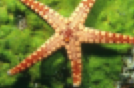
The second argument to the downsa program is the zoom factor, always a positive integer:
downsa a 9 masked.png downsa_max_9.png
downsa a 8 masked.png downsa_max_8.png
downsa a 7 masked.png downsa_max_7.png
downsa a 6 masked.png downsa_max_6.png
downsa a 5 masked.png downsa_max_5.png
downsa a 4 masked.png downsa_max_4.png
downsa a 3 masked.png downsa_max_3.png
downsa a 2 masked.png downsa_max_2.png
downsa a 1 masked.png downsa_max_1.png
The ntiply program is an inverse of downsa: it creates a larger image by replicating each pixel into a block of n×n. The dimensions of the images are multiplied by n, exactly.
downsa a 9 masked.png | ntiply 9 - ntiply_9.png
downsa a 8 masked.png | ntiply 8 - ntiply_8.png
downsa a 7 masked.png | ntiply 7 - ntiply_7.png
downsa a 6 masked.png | ntiply 6 - ntiply_6.png
downsa a 5 masked.png | ntiply 5 - ntiply_5.png
downsa a 4 masked.png | ntiply 4 - ntiply_4.png
downsa a 3 masked.png | ntiply 3 - ntiply_3.png
downsa a 2 masked.png | ntiply 2 - ntiply_2.png
downsa a 1 masked.png | ntiply 1 - ntiply_1.png
The upsa program is another inverse of downsa: it creates a larger image by interpolating the pixel values on a grid with n×n the resolution. Notice that an image of size W&ntimes;H is transformed into an image of size (nW-n)×(nH-n), because the interpolator needs values at both sides of the new samples. The second argument is the order of the spline used to interpolate:
downsa v 7 A.png A_downsa7.png
downsa v 7 A.png | upsa 7 0 - upsa_7_0.png    # nearest-neighbor interpolation
downsa v 7 A.png | upsa 7 1 - upsa_7_1.png    # piecewise linear
downsa v 7 A.png | upsa 7 2 - upsa_7_2.png    # bilinear
downsa v 7 A.png | upsa 7 3 - upsa_7_3.png    # bicubic
downsa v 7 A.png | upsa 7 -2 - upsa_7_-2.png  # bilinear with Quilez fading
downsa v 7 A.png | upsa 7 -3 - upsa_7_-3.png  # bicubic with Quilez fading
Notice that upsa with nearest-neighbor interpolation looks similar to ntiply, but it is not identical (the images have different size).
downsa v 20 b.jpg | upsa 20 0 - b_upsa_20.png
downsa v 20 b.jpg | ntiply 20 - b_ntiply_20.png
downsa v 20 b.jpg|upsa 20 0|GETPIXEL=0 plambda zero:240x240 - "x y(-10,-10)" -o b_upsabg_20.png
The program homwarp allows a finer control of the transformation: you get to specify the 9 coefficients of an arbitrary homography and the desired size of the output image. Notice that this generalizes upsa and ntiply but it does much more: it allows for arbitrary rotations and scalings.
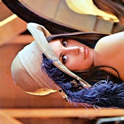
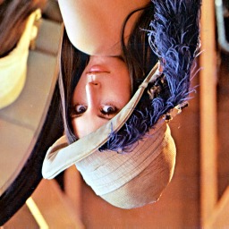
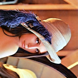
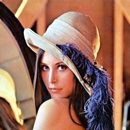
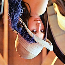
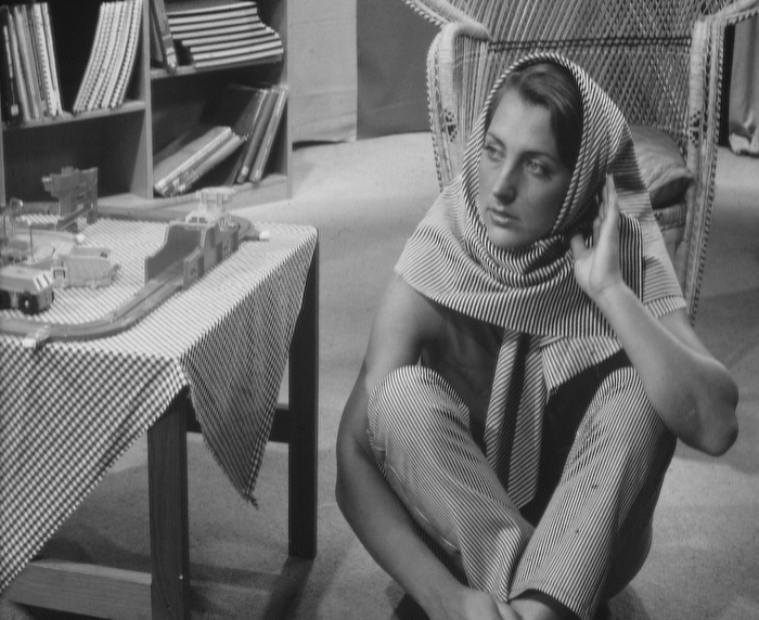
A very common particular case of rotations are those of straight angles. They are directly performed by the program imflip:
imflip r90       b.jpg b_r90.png
imflip r180      b.jpg b_r180.png
imflip r270      b.jpg b_r270.png
imflip leftright b.jpg b_leftright.png
imflip topdown   b.jpg b_topdown.png
imflip transpose b.jpg b_transpose.png
imflip posetrans b.jpg b_posetrans.png
imflip identity  b.jpg b_identity.png
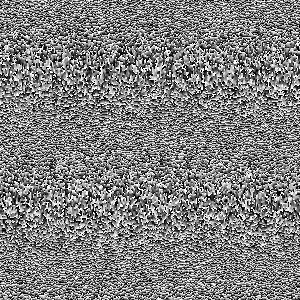
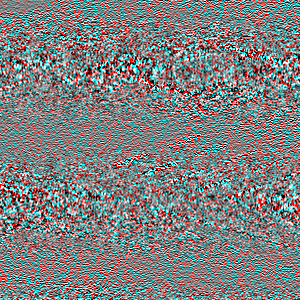
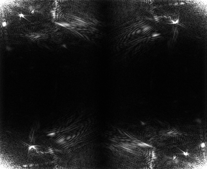
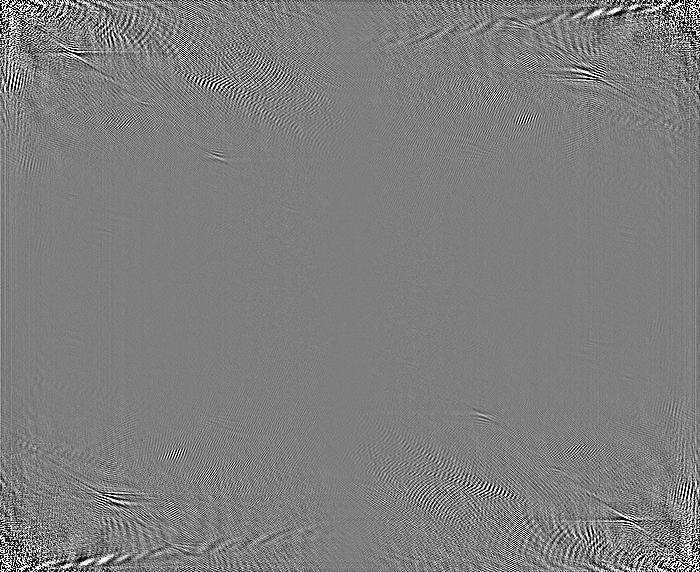
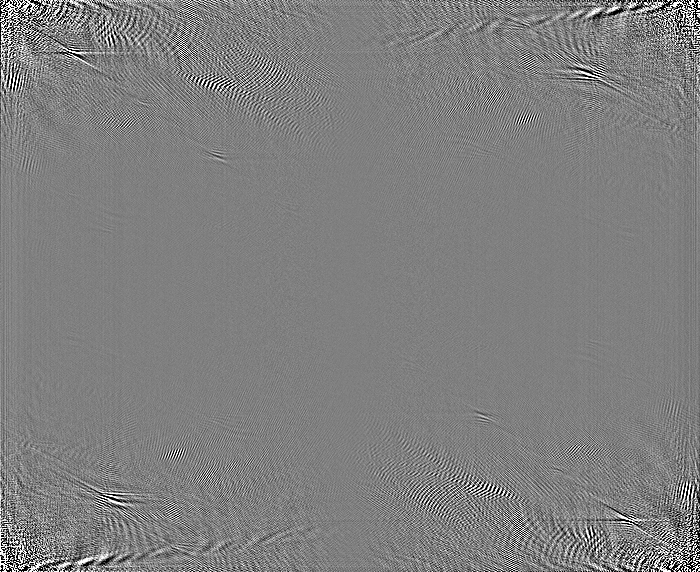
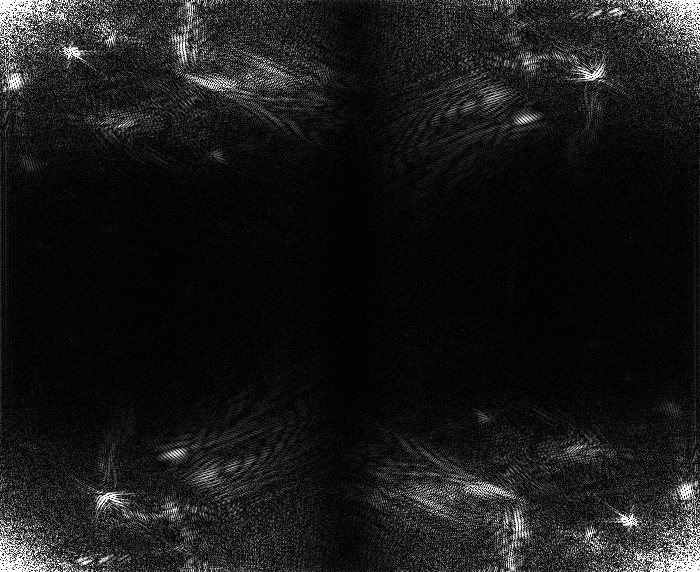
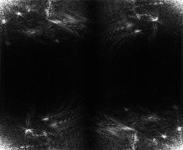
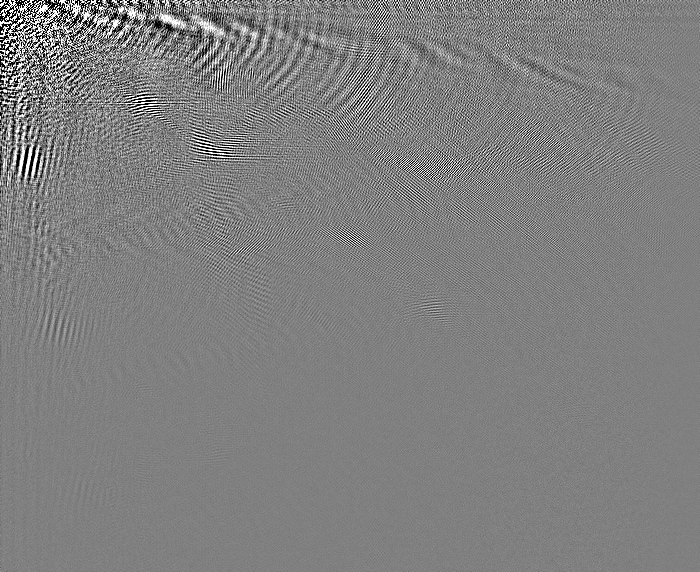
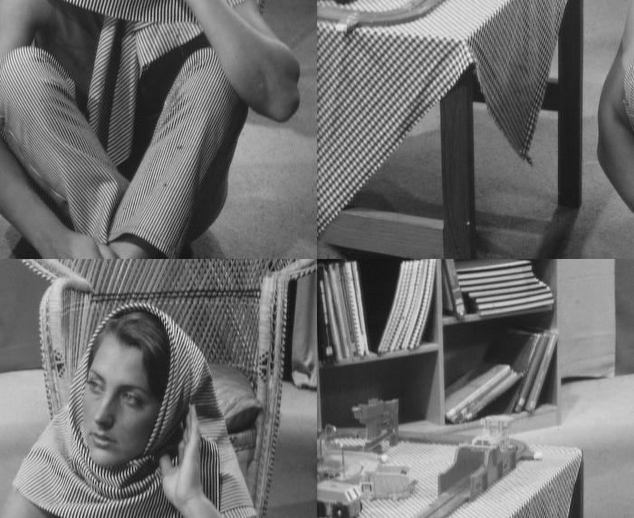
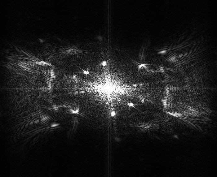
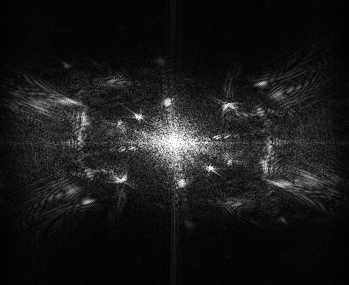
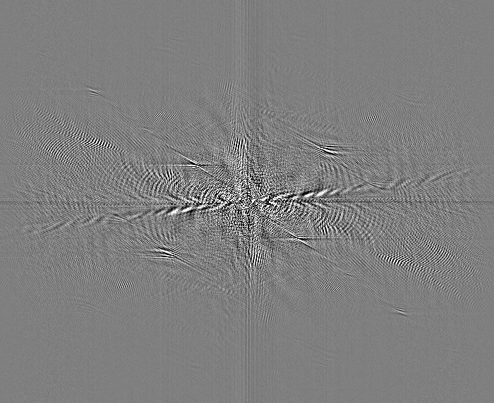
The fft, ifft, dct and dht programs are filters tha compute, respectively, the discrete Fourier transform, its inverse, the discrete cosine transform and the discrete Hartley transform. The DCT and the DHT are self-inverses, and the IFFT is the inverse of the FFT.
cat barb.png | fft | plambda vnorm       | qauto -p 1 - barb_dft_abs.png
cat barb.png | fft | plambda "x[0]"      | qauto -p 1 - barb_dft_re.png
cat barb.png | fft | plambda "x[1]"      | qauto -p 1 - barb_dft_im.png
cat barb.png | fft | plambda "x[0] fabs" | qauto -p 1 - barb_dft_are.png
cat barb.png | fft | plambda "x[1] fabs" | qauto -p 1 - barb_dft_aim.png
cat barb.png | dht                       | qauto -p 1 - barb_dht.png
cat barb.png | dht | plambda fabs        | qauto -p 1 - barb_dht_abs.png
cat barb.png | dct                       | qauto -p 1 - barb_dct.png
cat barb.png | dct | plambda fabs        | qauto -p 1 - barb_dct_abs.png
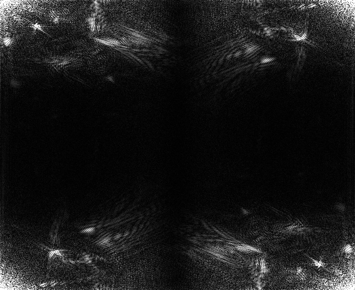
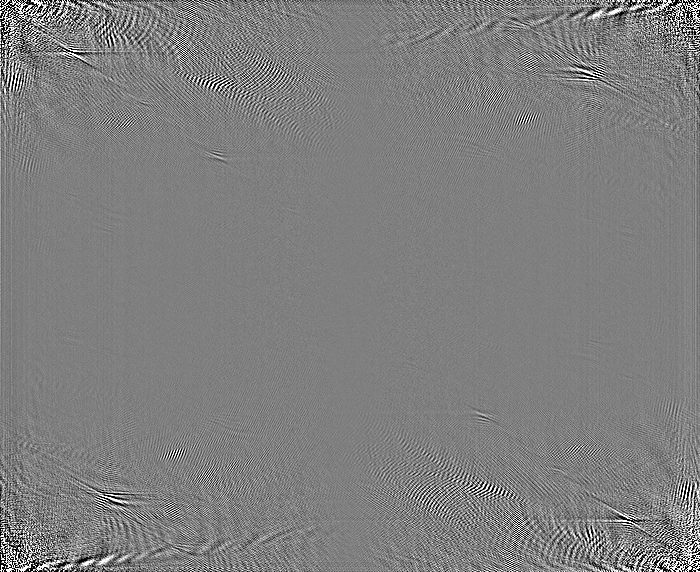
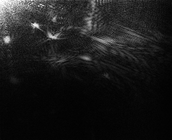
fftshift barb.png barb_s.png
cat barb.png | fft | plambda vnorm | fftshift | qauto -p 1 - barb_dft_s.png
cat barb.png | dht | plambda vnorm | fftshift | qauto -p 1 - barb_dht_abs_s.png
cat barb.png | dht                 | fftshift | qauto -p 1 - barb_dht_s.png
end